Financial Mathematics
Introduction and Motivation
Motivation
From the Actuaries Institute:
“Actuaries evaluate risk and opportunity - applying mathematical, statistical, economic and financial analyses to a wide range of business problems.”
A key concept here is financial; most of an actuary’s work relates in some way or another to money, such as insurance claims, superannuation benefits, investment returns, etc. Understanding the time value of money is crucial: $1,000 today does not hold the same value as $1,000 in 20 years…
Overview
Financial mathematics are typically not an end in itself but a fundamental tool that actuaries need. This week covers the valuation of known future cash-flows. Another difficulty in actuarial studies is that cash flows related to losses are by nature uncertain. In-depth coverage is provided in the course ACTL2111: Financial Mathematics.
Historically, actuaries developed the application of the mathematics of finance to insurance problems as early as the 1700s.
Some Applications
- Personal and Housing Loans
- Personal loan - usually with level repayments, “flat” fixed interest rates (3 to 5 years)
- Housing loan - level repayments of loan principal and interest (20 to 30 years), variable interest rates in Australia, flexible repayments
- Fixed and Floating Interest Securities (Bonds)
- Repayments of interest (coupons) and face value on maturity
- Includes government bonds, corporate bonds
Compound Interest
“Money makes money. And the money that money makes, makes money.” - Benjamin Franklin
“The most powerful force in the universe is compound interest.” - Albert Einstein (possibly apocryphal, see Snopes)
Definitions
- Nominal Interest Rate - Interest rates are normally QUOTED as per annum percentage nominal rates.
- Effective Interest Rate per Period - Let $j^{(m)}$ denote the per annum nominal interest rate with $m$ periods. The effective interest rate per period is calculated as: $r = \frac{j^{(m)}}{m}$
Continuous Compounding
- The
continuously compounded interest rateis the nominal interest rate obtained when the compounding frequency is increased to infinity. - Known as the force of interest, with the mathematical constant $e$ discovered by Jacob Bernoulli in 1683.
- For an annual effective rate of 10% p.a., the continuously compounded interest rate is approximately 9.530%, calculated as:
\delta = \ln[1 + j] = \ln[1.1] = 0.09531
Annuities and Actuarial Notation
Time Certain Annuity
A time certain annuity is a stream of level payments, happening at regular intervals. Assuming a constant interest rate, the symbol $a_{\overline{n}|}$ represents the Present Value (PV) of $n$ payments of 1, payable in arrears (at the end of each period).
- Let $i$ be the interest rate effective per period.
The computation of $a_{\overline{n}|}$ can be expressed as:
a_{\overline{n}|} = \sum_{j=1}^{n}\left(\frac{1}{1+i}\right)^j
= \frac{1}{1+i} \left[\frac{1-\left(\frac{1}{1+i}\right)^n}{1-\left(\frac{1}{1+i}\right)}\right]
= \frac{1-\left(\frac{1}{1+i}\right)^n}{i}
= \frac{1-v^n}{i}, \text{where } v \equiv \frac{1}{1+i}
Time Certain Annuity - Example
Example 4.7: Calculate $a_{\overline{n}|}$ at an interest rate of $i = 0.01$ per period.
Solution:
a_{\overline{n}|} = \frac{1-v^n}{i}
= \frac{1-\left(\frac{1}{1.01}\right)^{10}}{0.01}
= 9.4713
Annuity Due - Payments in Advance
- Actuarial notation: place “double-dots” over the annuity symbol to indicate (n) payments made in advance: $\ddot{a}_{\overline{n}|}$.
- This symbol then represents the Present Value of $n$ payments of 1, if the first payment is made immediately:
\ddot{a}_{\overline{n}|} = \sum_{j=0}^{n-1}(\frac{1}{1+i})^j
The relationship between $a_{\overline{n}|}$ and $\ddot{a}_{\overline{n}|}$ can be defined as:
\ddot{a}_{\overline{n}|}  = \left[\frac{1-\left(\frac{1}{1+i}\right)^n}{1-\left(\frac{1}{1+i}\right)}\right]
= (1+i) \left[\frac{1-\left(\frac{1}{1+i}\right)^n}{i}\right]
= (1+i) a_{\overline{n}|}
But did we really need those calculations?
Annuity Due - Example
Example 4.8: Calculate the present value of a 5 year annuity due at 6% per annum.
Solution:
\ddot{a}_{\overline{n}|} = (1.06) \left[\frac{1-\left(\frac{1}{1.06}\right)^5}{0.06}\right]
= 4.4651
Fixed-Income Instruments
Types of Fixed-Income Instruments
Fixed-income instruments can be categorized into three main types:
- Discount Instruments: Examples include zero-coupon bonds.
- Periodic Interest Instruments: Examples include regular coupon bonds.
- Level Payment Instruments: Examples include mortgages.
Source: CFA Level 1 Curriculum 2024: Quantitative Methods
Time Value of Money Principles
The relationship between a current or present value (PV) and future value (FV) of a cash flow, given a discount rate (r) per period and (t) compounding periods, is defined as:
- Future Value:
FV_t = PV \times (1 + r)^t - Present Value:
PV = \frac{FV_t}{(1 + r)^t}
When compounding continuously:
- Future Value with Continuous Compounding:
FV_t = PV \times e^{rt} - Present Value with Continuous Compounding:
PV_t = FV \times e^{-rt}
Coupon Bond Cash Flow Diagram
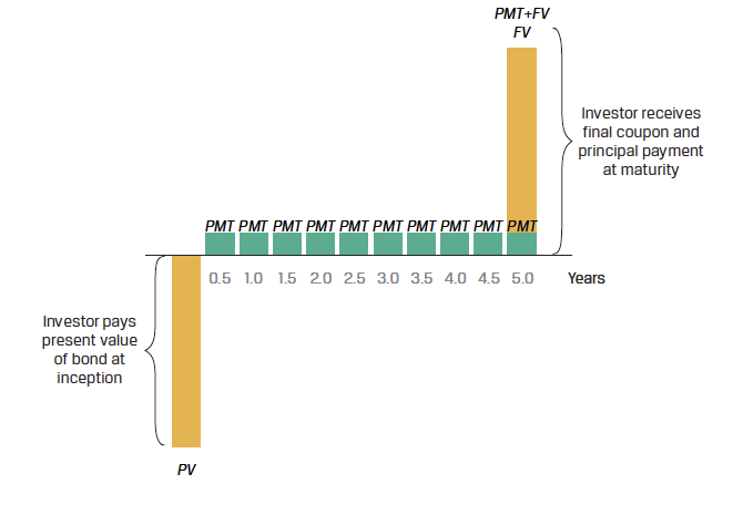
Figure: Coupon Bond cash flow diagram.
Pricing a Coupon Bond
Pricing a coupon bond extends the single cash flow calculation for a discount bond to a general formula for calculating a bond’s price (PV) given the market discount rate on a coupon date:
PV_{\text{Coupon Bond}} = \frac{PMT_1}{(1 + r)^1} + \frac{PMT_2}{(1 + r)^2} + \ldots + \frac{PMT_N + FV_N}{(1 + r)^N}
This formula accounts for all periodic payments (PMT) and the final payment of the principal (FVN) at maturity.
Republic of India Semiannual Coupon Bond - Overview
Bond Details
- Duration: 20 years
- Coupon Rate: 6.70% (Annualized)
- Yield to Maturity (YTM): 6.70%
- Payment Frequency: Semiannual
Coupon Payments
- Semiannual Payment (PMT): INR3.35 $(= 6.70/2)$
- Periodic Discount Rate: 3.35\% $(= 6.70/2)$
Pricing Calculation
Pricing at Issuance:
- Principal: INR100
Present Value Calculation:
PV = \frac{3.35}{1.0335} + \frac{3.35}{1.0335^2} + \ldots + \frac{103.35}{1.0335^{40}}
Explanation:
- Since the coupon rate equals the YTM, the present value (PV) of the bond at issuance is expected to be INR100.
- This calculation assumes that each coupon payment and the final principal are discounted back to their present value using the semiannual discount rate.
Perpetual Bonds
A perpetual bond is a type of coupon bond with no stated maturity date, providing continuous cash flows indefinitely:
PV_{\text{Perpetual Bond}} = \frac{PMT}{r}
This formula simplifies the present value calculation for perpetual bonds, assuming the rate $r$ is positive.
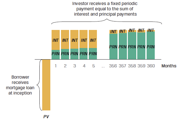
Annuity Instruments: Mortgage Example
Fixed-income instruments with level payments, such as mortgages, combine interest and principal cash flows throughout their duration.
Calculating Annuity Cash Flows
The periodic annuity cash flow (PMT), occurring at the end of each period, can be calculated using the formula:
PMT = \frac{PV \cdot r}{1 - (1 + r)^{-t}}
Where:
- PMT: periodic cash flow
- r: market interest rate per period
- PV: present value or principal amount of the loan or bond
- t: number of payment periods
Using Actuarial Notations:
\frac{PV}{PMT} = a_{\overline{n}|}
Where:
- $i$ is the interest rate per period $(= r)$
- $n$ is the total number of payment periods $(= t)$
Example: Mortgage Cash Flows
An investor seeks a fixed-rate 30-year mortgage loan to finance 80% of the purchase price of USD 1,000,000 for a residential building.
Calculate the investor’s monthly payment:
- Annual mortgage rate: 5.25%
- Monthly rate $r$: $0.4375 = \frac{5.25}{12}$
- Number of payments $t$: 360
- Principal Value $PV$: $USD 800,000 = 0.8 \times USD 1,000,000$
PMT = \text{USD } 4,417.63 = \frac{0.4375\% \times USD 800,000}{1 - (1 + 0.4375\%)^{-360}}
Interest and Principal Breakdown
Month 1:
- Interest: USD 3,500 = USD 800,000 $\times$ 0.4375\%
- Principal Amortization: USD 917.63 = USD 4,417.63 - USD 3,500
- Remaining Principal: USD 799,082.37 = USD 800,000 - USD 917.63
Month 2:
- Interest: USD 3,495.99 = USD 799,082.37 $\times$ 0.4375\%
- Principal Amortization: USD 921.64 = USD 4,417.63 - USD 3,495.99
- Remaining Principal: USD 798,160.73 = USD 799,082.37 - USD 921.64
Although the periodic payment is constant, the proportion of interest per payment declines, and the principal amortization rises over time.